
An Introduction to Multiple Linear Regression (MLR) in R
Discover the essentials of multiple linear regression in R, through a practical “Performance Index” dataset.
What Is Predictive Modelling?
Predictive modeling involves creating a statistical model to predict or estimate the probability of an outcome. These models are typically developed using historical or purposely collected data. Predictive analytics has applications across many domains, including finance, insurance, telecommunications, retail, healthcare, and sports.
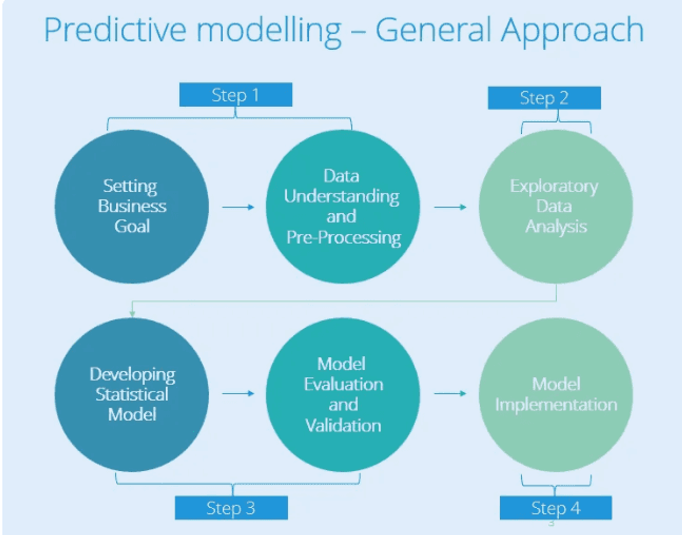
Predictive Modeling – General Approach
- Setting the Business Goal
- Data Understanding and Pre-Processing
- Exploratory Data Analysis
- Developing Statistical Model
- Model Evaluation and Validation
- Model Implementation
Multiple Linear Regression Introduction
Multiple linear regression (MLR) is used to explain the relationship between one continuous dependent variable and two or more independent variables, which can be continuous or categorical. The variable we want to predict (or model) is called the dependent variable, while the independent variables (also known as explanatory variables or predictors) are those used to predict the outcome.
Example: If the goal is to predict a house’s price (dependent variable), potential independent variables could include its area, location, air quality index, or distance from the airport.
Multiple Linear Regression: Statistical Model
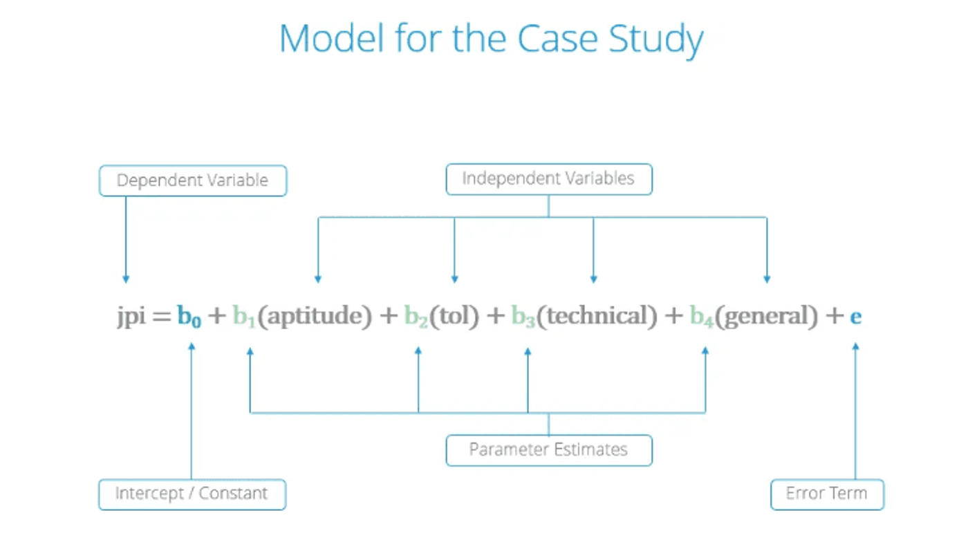
Y = β0 + β1X1 + β2X2 + ⋯ + βpXp + ε
- Y: Dependent variable
- X1, X2, …, Xp: Independent variables
- β0, β1, …, βp: Parameters (coefficients)
- ε: Random error component
MLR requires that the model be linear in the parameters (though the predictors themselves can be numeric or categorical). Parameter estimates are often found using the Least Squares Method, which minimizes the sum of squared residuals.
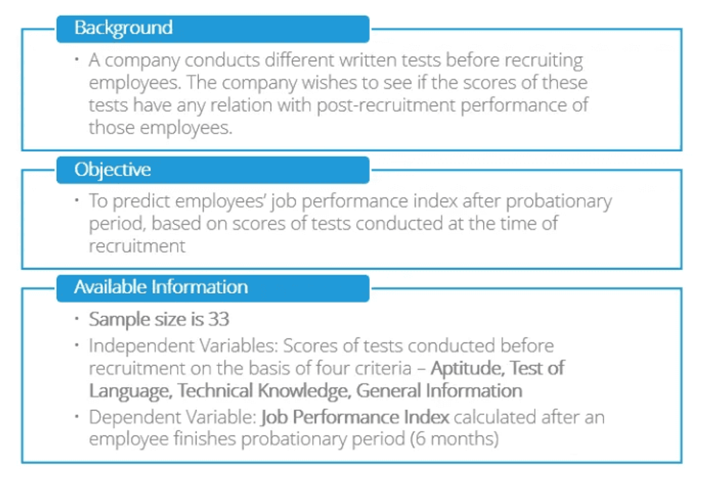
Case Study – Modeling Job Performance Index
This case study uses a dataset called Performance Index, containing:
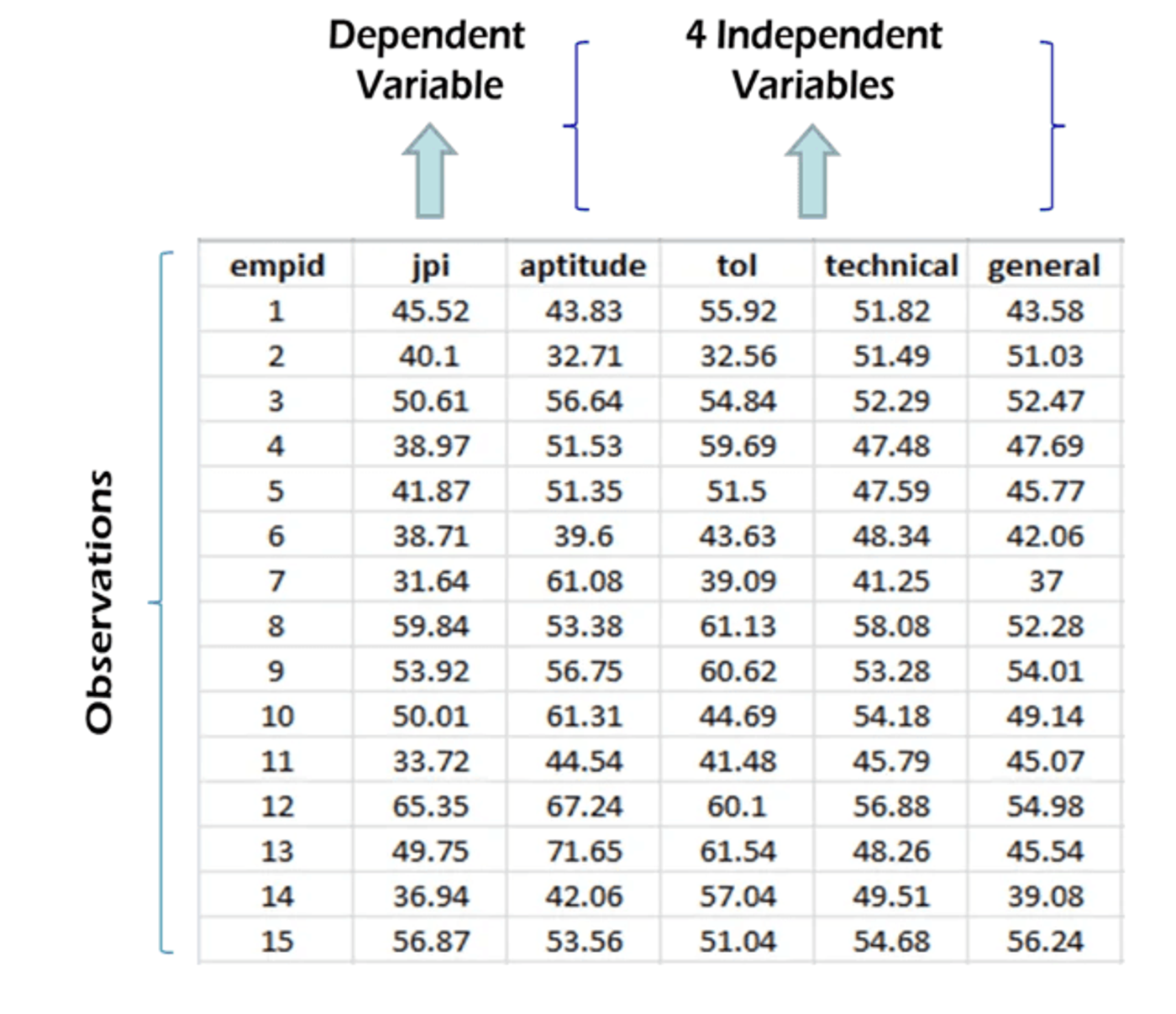
- jpi: Job Performance Index (dependent variable)
- aptitude: Aptitude test score
- tol: Test of language score
- technical: Technical knowledge score
- general: General information score
Data Snapshot
| Columns | Description | Type | Measurement | Possible values |
|---|---|---|---|---|
| empid | Employee ID | integer | - | - |
| jpi | Job performance Index | numeric | - | positive values |
| aptitude | Aptitude score | numeric | - | positive values |
| tol | Test of Language | numeric | - | positive values |
| technical | Technical Knowledge | numeric | - | positive values |
| general | General Information | numeric | - | positive values |
Below is a snippet of how we might load and inspect the dataset in R.
# Reading the Performance Index dataset
performance_data <- read.csv("Performance Index.csv")

# View the first few rows
head(performance_data)

# Check basic summary statistics
summary(performance_data)
Parameter Estimation Using the Least Squares Method
| Parameters | Coefficients |
|---|---|
| Intercept | -54.2822 |
| aptitude | 0.3236 |
| tol | 0.0334 |
| technical | 1.0955 |
| general | 0.5368 |
If we denote Job Performance Index as jpi, then one possible model from the data is:

Parameter Estimation Using lm() in R
Model Fit
#Model Fit
model <- lm(jpi ~ aptitude + tol + technical + general, data = performance_data)
Output
#Output
summary(model)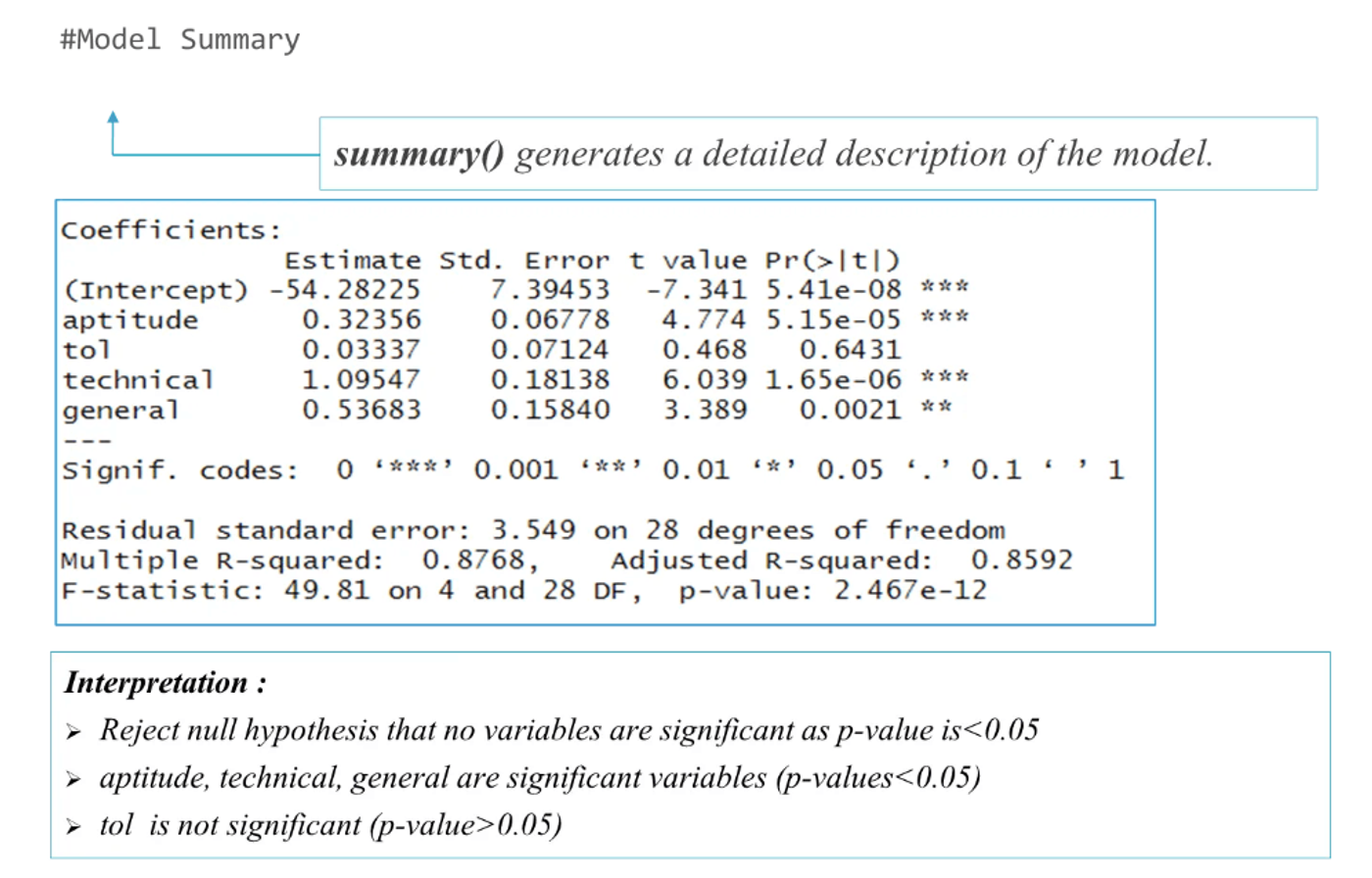
Interpretation of Partial Regression Coefficients
Each coefficient βi tells us how much jpi changes with a one-unit increase in the corresponding predictor, holding all other variables constant. For instance, if the coefficient for aptitude is 0.3236, then a 1-point increase in the aptitude score (assuming everything else is fixed) increases the job performance index by 0.3236.
Individual Testing – Using t Test
To test which variables are significant:
- Null Hypothesis (H0): βi = 0
- Alternate Hypothesis (H1): βi ≠ 0
The summary(model) output provides p-values for each coefficient. Typically, a p-value < 0.05 suggests that the variable is significant.
| Parameters | Coefficients | Standard Error | t statistic | p-value |
|---|---|---|---|---|
| Intercept | -54.2822 | 7.3945 | -7.3409 | 0.0000 |
| aptitude | 0.3236 | 0.0678 | 4.7737 | 0.0001 |
| tol | 0.0334 | 0.0712 | 0.4684 | 0.6431 |
| technical | 1.0955 | 0.1814 | 6.0395 | 0.0000 |
| general | 0.5368 | 0.1584 | 3.3890 | 0.0021 |
Measure of Goodness of Fit – R²
R² indicates the proportion of variation in the dependent variable (jpi) explained by the independent variables. Higher R² values imply a better fit. An adjusted R² also accounts for the number of predictors in the model.
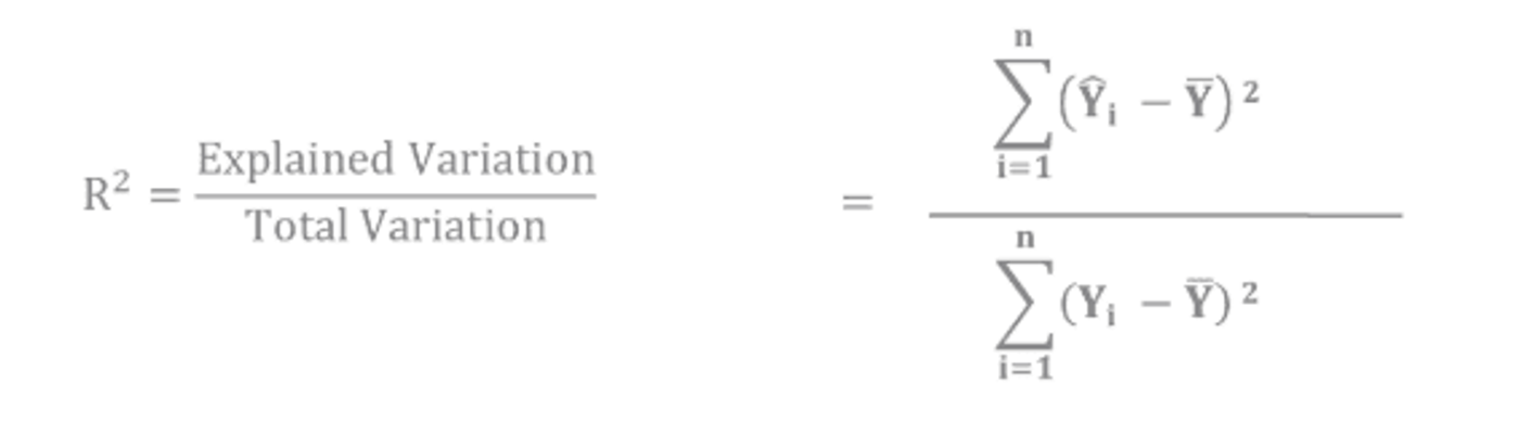
The adjusted R-squared is a modified version of R-squared that has been adjusted for the number of predictors in the modelling.

Summary Output
- Significant variables are aptitude, technical, and general since their p-values are < 0.05.
- Insignificant variable is tol, as its p-value exceeds 0.05.
- An R-squared of 0.88 suggests that 88% of the variation in job performance is explained by these predictors.
- Interpretation: Increasing
aptitudeby 1 unit, while holding other variables constant, increasesjpiby approximately its parameter estimate. The same logic applies totechnicalandgeneral.
Fitted Values and Residuals
Once you have the estimated model, you can compute fitted values and residuals:
Adding Fitted Values and Residuals to the Original Dataset
# Adding Fitted Values and Residuals
performance_data$pred <- fitted(model)
performance_data$resi <- resid(model)

head(performance_data)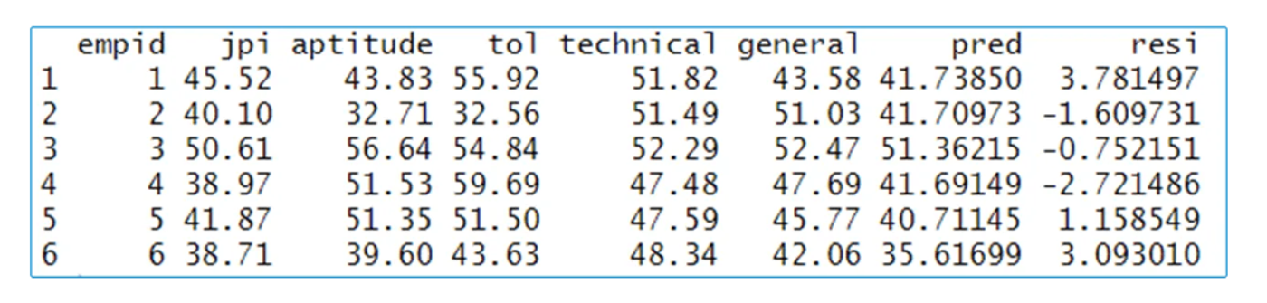
Predictions for a New Dataset
When you have new data with the same independent variables, you can generate predictions:
# Importing New Dataset
new_data <- read.csv("Performance Index new.csv")

# Generating predictions
new_data$pred <- predict(model, newdata = new_data)

head(new_data)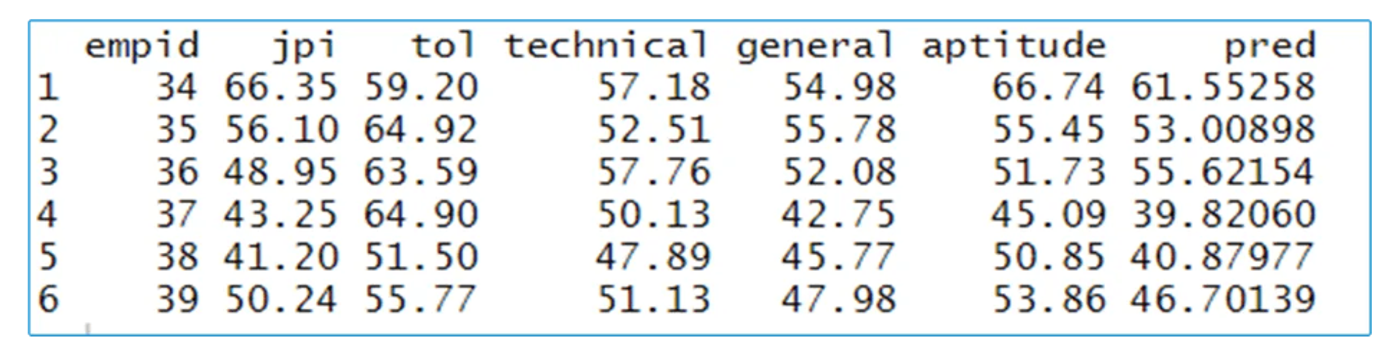
Important: Ensure that the new dataset has all the independent variables used in the model, with matching column names.
Multiple Linear Regression: Assumptions & Diagnostics
We built a multiple linear regression model to predict jpi (Job Performance Index) from four predictors in the Performance Index dataset:
aptitudetol(test of language)technicalgeneral
In this continuation, we will check the assumptions of multiple linear regression—multicollinearity and the normality of errors—and illustrate residual analysis techniques. Such checks are essential to ensure valid model interpretations and reliable predictions.
Problem of Multicollinearity
Multicollinearity arises when two or more independent variables in a regression model exhibit a strong linear relationship. This leads to:
- Highly unstable model parameters: The standard errors of the coefficients become inflated, making them unreliable.
- Potentially poor out-of-sample predictions: The model might fail to generalize accurately.
Hence, detecting and handling multicollinearity is an important step in regression.
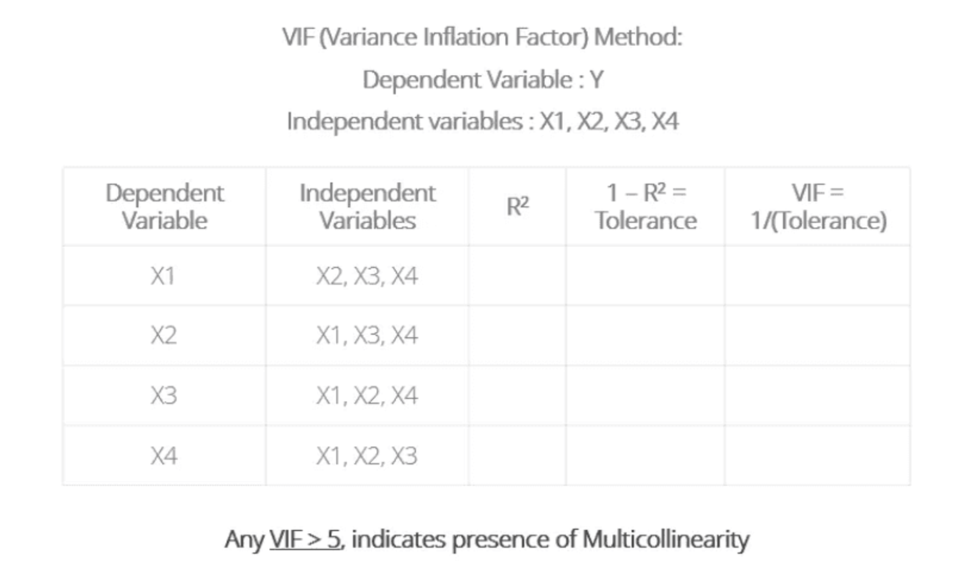
Detecting Multicollinearity Through VIF
The Variance Inflation Factor (VIF) is a common way to detect multicollinearity. A VIF > 5 (some use a threshold of 10) can indicate problematic multicollinearity.
Detecting Multicollinearity in R
# Assume the Performance Index data is loaded as performance_data.
# We fit the same model as before:

model <- lm(jpi ~ aptitude + tol + technical + general, data = performance_data)

# To calculate VIF, we use the 'car' package:
# install.packages("car") # Uncomment if not installed
library(car)

vif_values <- vif(model)
vif_values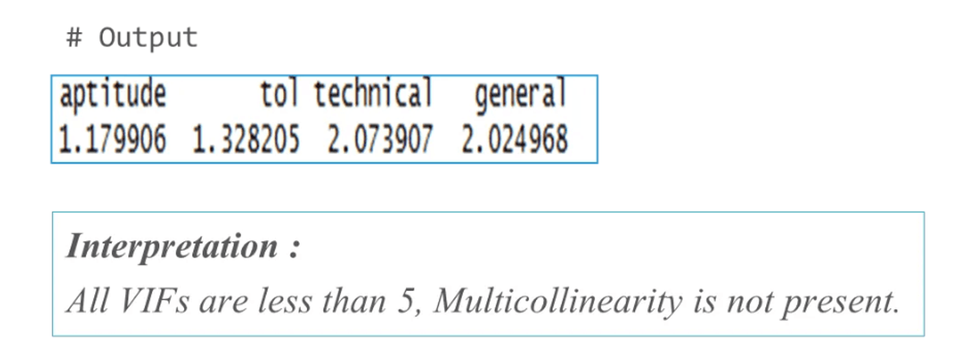
If one or more VIF values exceed 5, you are likely dealing with multicollinearity.
Multicollinearity – Remedial Measures
Possible solutions include:
- Removing one or more correlated independent variables
- Combining correlated predictors via dimensionality reduction (e.g., Principal Component Analysis)
- Collecting more data to stabilize parameter estimates
Residual Analysis
Residuals represent the difference between the observed and predicted values:
Residual = Observed Value − Predicted Value
A thorough residual analysis is vital for checking assumptions:
- Errors follow a Normal Distribution (Normality of errors)
- Homoscedasticity (Constant variance of residuals)
- No obvious patterns or autocorrelation
Normality of Errors
Multiple linear regression assumes that the errors (residuals) follow a normal distribution. If this assumption is severely violated, the p-values and confidence intervals (based on t and F distributions) can become unreliable.
Residual Analysis for the Performance Index Data
Continuing with our Performance Index model:
- Get the fitted values and residuals.
- Analyze their distribution.
# Calculate residuals
resids <- residuals(model)

# Plot residuals vs. predicted values
plot(fitted(model), resids,
     xlab = "Fitted Values (Predicted jpi)",
     ylab = "Residuals",
     main = "Residuals vs. Predicted")
abline(h = 0, col = "red")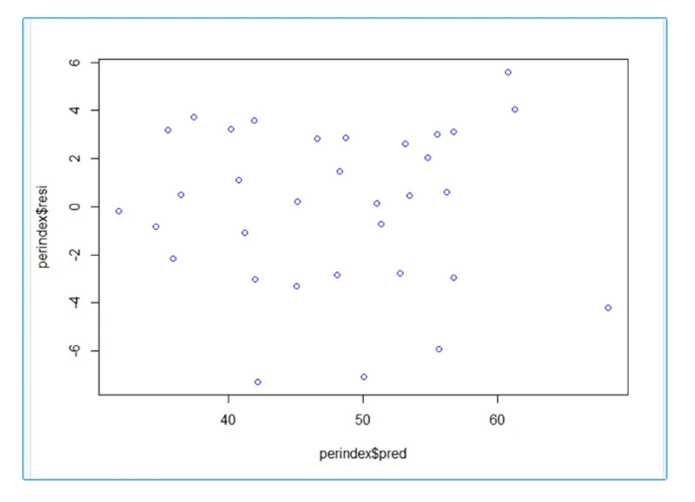
Interpretation:
Residuals in our model are randomly distributed which indicates presence of Homoscedasticity
A random scatter around zero is generally good; patterns or funnel-shaped spreads can indicate issues like heteroscedasticity or non-linearity.
Normality Checks
- Q-Q Plot
- Shapiro-Wilk Test
- Kolmogorov-Smirnov (KS) Test
Q-Q Plot
The Q-Q plot compares sample quantiles of the residuals to the theoretical quantiles of a normal distribution. If points lie roughly on a straight line, the errors are likely normally distributed.
qqnorm(resids, main = "Normal Q-Q Plot of Residuals")
qqline(resids, col = "red")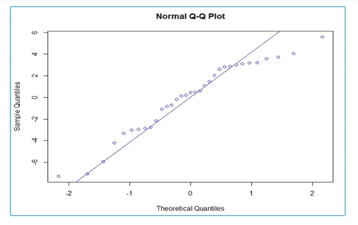
Interpretation:
Most of these points are close to the line except few values indicating no serious deviation from Normality.
Shapiro-Wilk Test
shapiro.test(resids)A p-value > 0.05 suggests we do not reject the hypothesis that the residuals are normally distributed.
Absence of Normality – Remedial Measures
If the residuals are not normally distributed, we can apply transformations to the dependent variable, such as a log transform. More generally, a Box-Cox transformation can be used, where R will attempt to find an optimal exponent (λ).
# install.packages("MASS") # Uncomment if not installed
library(MASS)
boxcox(model)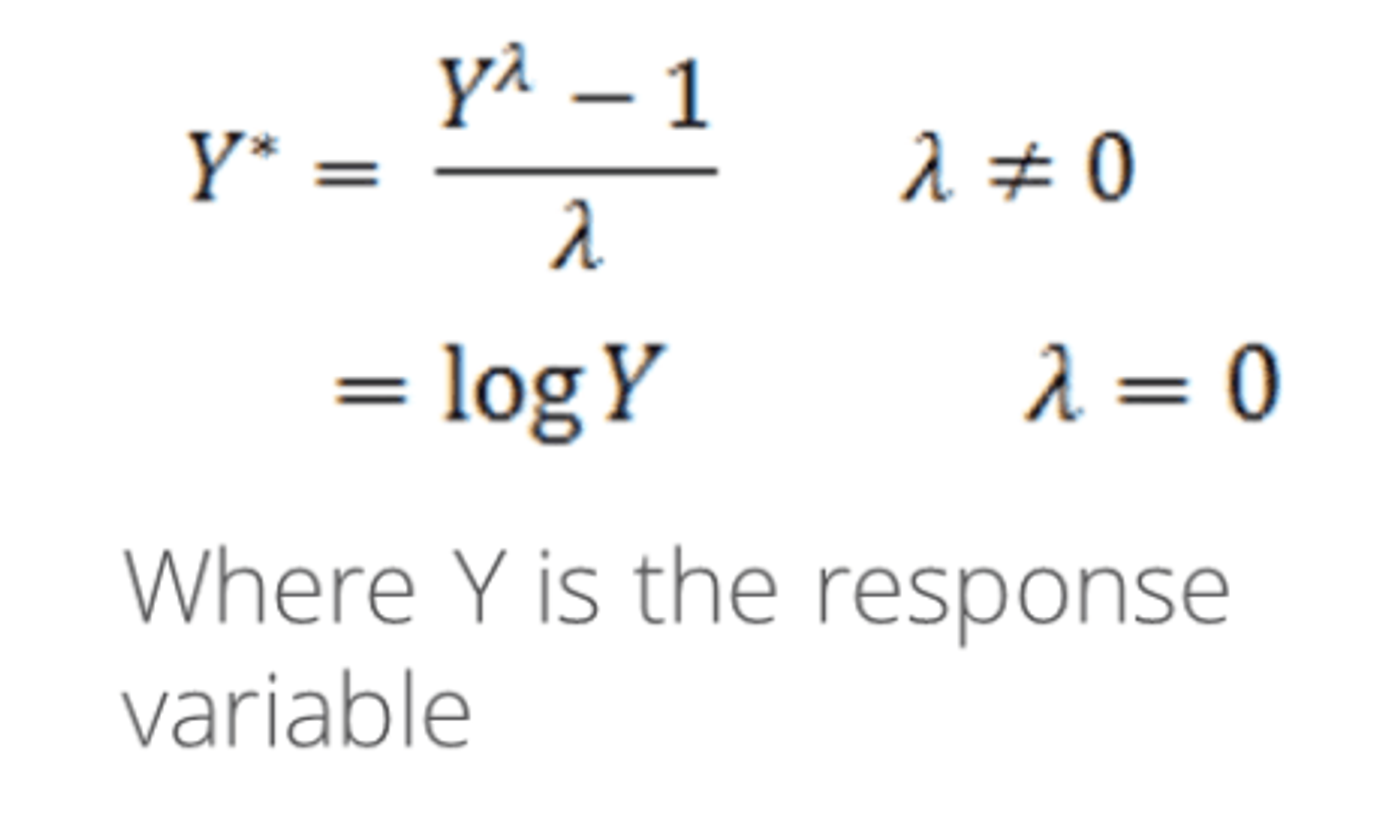
Key takeaways
- Fit the model with
lm(), then evaluate its coefficients, their significance (t-tests) and the model fit (R²). - In the Performance Index case study, aptitude, technical and general are significant (p < 0.05) and tol is not; an R² of 0.88 means the predictors explain 88% of the variation in job performance.
- The fitted model gives fitted values and residuals, and predicts new data that has all the independent variables with matching column names.
- Check multicollinearity with VIFs: values above 5 suggest removing or combining correlated variables.
- Check the residuals with a residuals-vs-fitted plot, a Q-Q plot and the Shapiro-Wilk test; if the errors are not normal, try a transformation such as Box-Cox.
By following these steps—business understanding, data exploration, model building, and evaluation—you can create robust predictive models to inform data-driven decisions.
By examining multicollinearity (via VIF) and residuals (via diagnostic plots and normality tests), you ensure that the multiple linear regression model for the Performance Index data remains trustworthy. Addressing issues like high correlation among predictors or non-normal errors can greatly improve the model’s reliability and predictive power.