Binary Logistic Regression in Python

Binary logistic regression models the relationship between a set of independent variables and a binary dependent variable. It is useful when the dependent variable is dichotomous in nature—for example: death or survival, absence or presence, pass or fail. In logistic regression, the dependent variable is a binary variable coded as 1 (yes, success, etc.) or 0 (no, failure, etc.). The logistic regression model essentially predicts P(Y=1) as a function of the independent variables X. The independent variables can be categorical or continuous (e.g., gender, age, income, region, and so on). Binary logistic regression models a dependent variable as a logit of p, where p is the probability that the dependent variable takes the value “1”.

Statistical Model – For k Predictors

The statistical model in binary logistic regression can be written as follows:

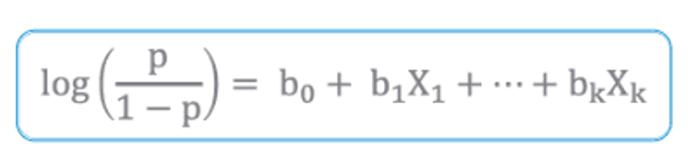
where

• p: Probability that Y=1 given X
• Y: Dependent Variable
• X1, X2, …, Xk: Independent Variables
• b0, b1, …, bk: Parameters (coefficients) of the model

The parameters (b0 to bk) are typically estimated using the maximum likelihood method. The left-hand side of the equation ranges from −∞ to +∞.

Case Study – Modeling Loan Defaults

To illustrate binary logistic regression, consider a bank’s scenario:

• The bank has demographic and transactional data of its loan customers.
• The goal is to develop a model predicting whether a customer will default or not on a new loan.
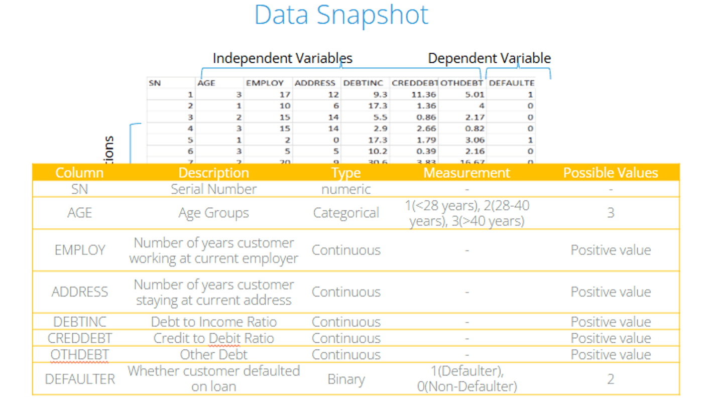
• We have a sample of 700 loan customers. The independent variables used are: Age group, Years at current address, Years at current employer, Debt to income ratio, Credit card debt and Other debt.

All these are collected at loan application. The dependent variable is the observed status (1 = defaulter, 0 = not defaulter) after the loan is disbursed.

Below is a snapshot of the data. The dependent variable is binary, while the independent variables are a mix of categorical and continuous types.

Importing and Inspecting the Data

import pandas as pd

# Import data and check data structure
bankloan = pd.read_csv('BANK LOAN.csv')
bankloan.info()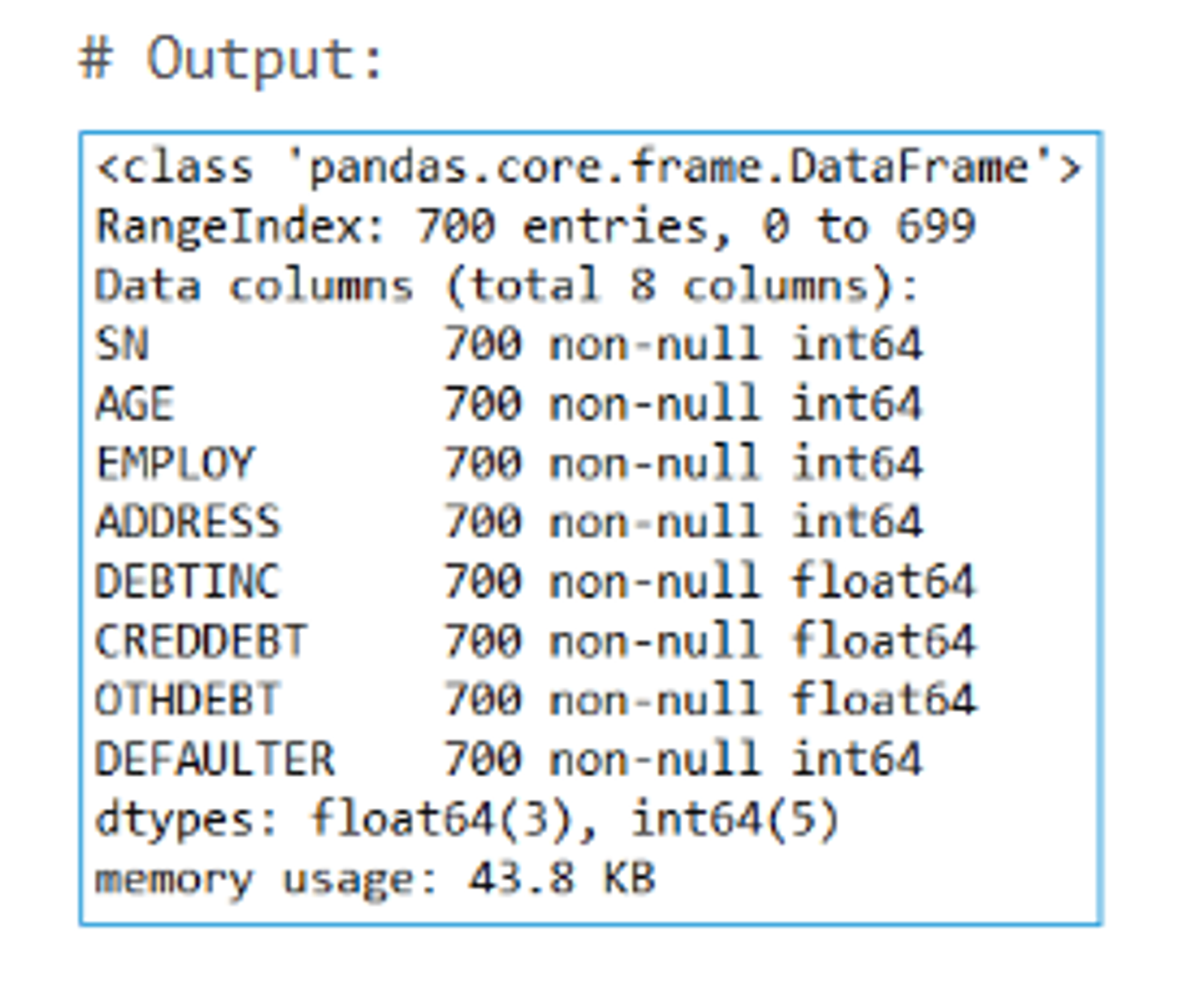

You might notice from the output that Age appears as an integer, but for our analysis, we need it to be a categorical variable (since we’re considering age groups). If we leave Age as a numeric variable, Python will treat it incorrectly as a continuous variable.

# Change ‘AGE’ variable into categorical
bankloan['AGE'] = bankloan['AGE'].astype('category')
bankloan.info()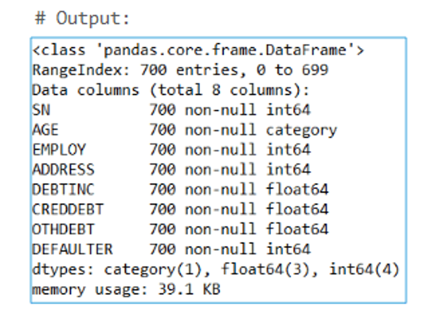

Fitting the Logistic Regression Model

In a logistic regression, we use the logit link function. Below is the initial model that includes all the variables we want to test:

import statsmodels.formula.api as smf

riskmodel = smf.logit(
    formula='DEFAULTER ~ AGE + EMPLOY + ADDRESS + DEBTINC + CREDDEBT + OTHDEBT',
    data=bankloan
).fit()

print(riskmodel.summary())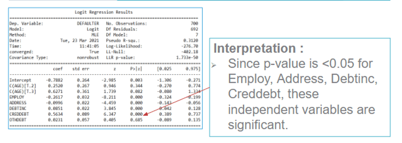

From the summary, we can see the significance (p-values) of each variable. The variables EMPLOY, ADDRESS, DEBTINC, and CREDDEBT are statistically significant (p-value < 0.05).

Re-running the Logistic Regression With Significant Variables

We now refine our model by dropping the insignificant variables:

riskmodel = smf.logit(
    formula='DEFAULTER ~ EMPLOY + ADDRESS + DEBTINC + CREDDEBT',
    data=bankloan
).fit()

print(riskmodel.summary())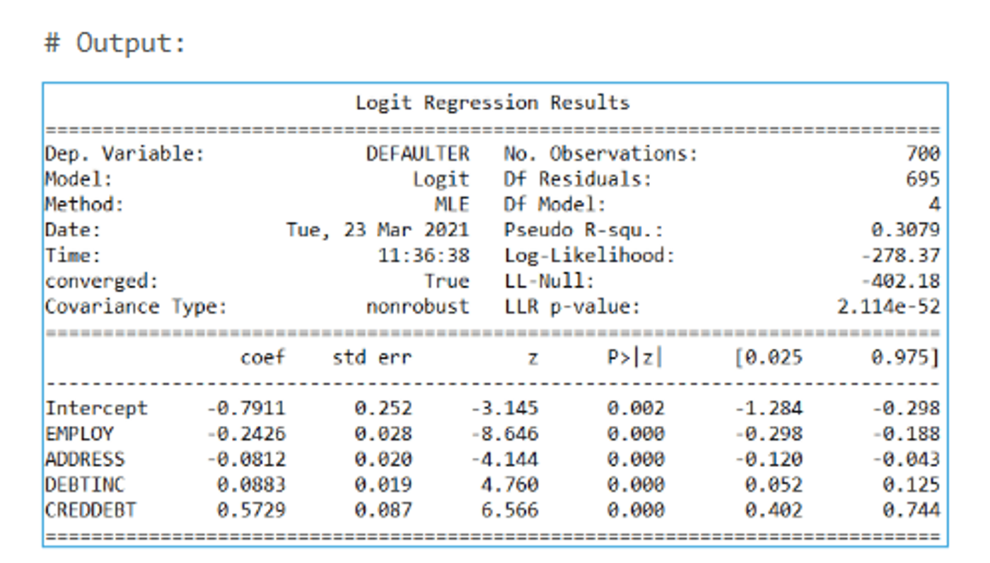

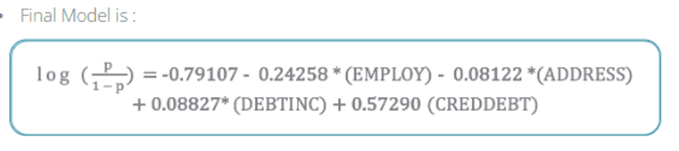
In this refined output, all the independent variables are significant, and the signs of the coefficients make sense. This final model can be used for further analysis.

Odds Ratios in Python

Odds ratios help interpret the effect of each independent variable on the probability of being a defaulter. After fitting the final model, we can obtain the parameter estimates along with confidence intervals, and then exponentiate (antilog) those estimates to get odds ratios.

import numpy as np

conf = riskmodel.conf_int()   # confidence intervals for parameters
conf['OR'] = riskmodel.params # model parameter estimates
conf.columns = ['2.5%', '97.5%', 'OR']

print(np.exp(conf))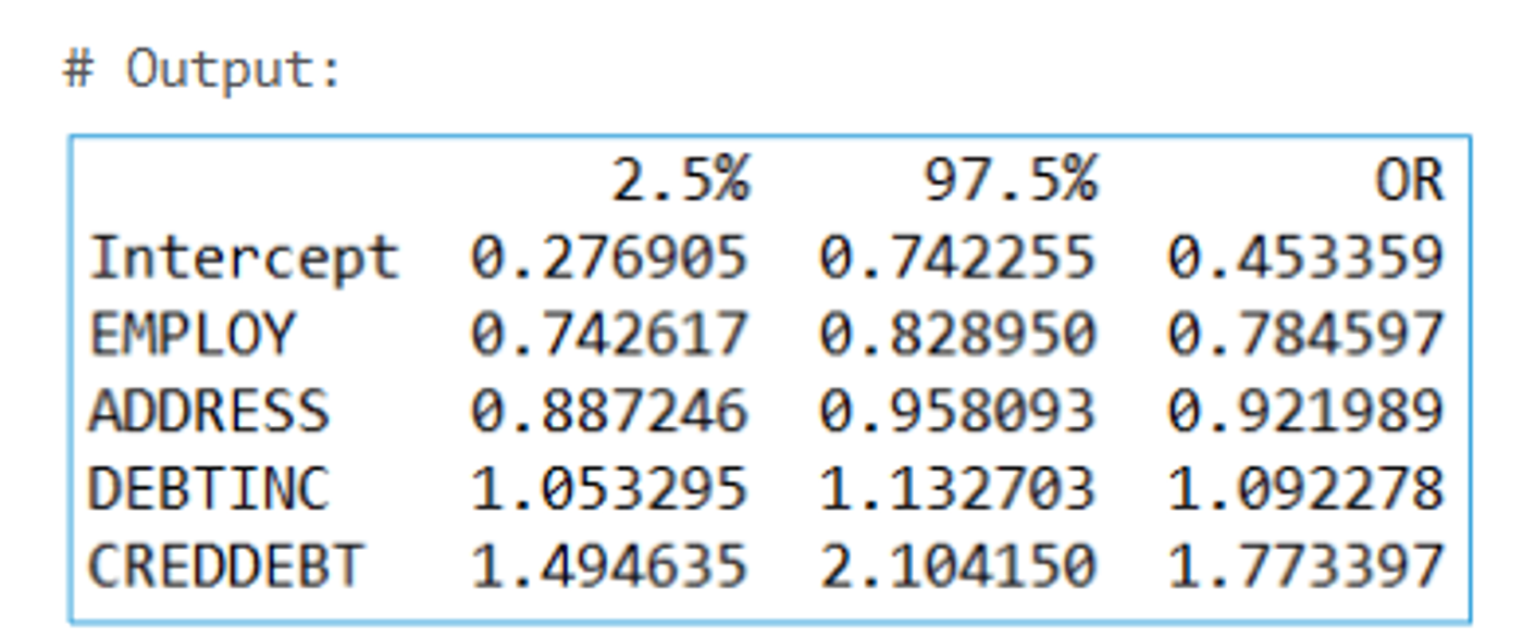

If an odds ratio’s confidence interval does not include 1, that variable is considered significant. For example, if CREDDEBT has an odds ratio of 1.77, then for a one-unit increase in CREDDEBT, the odds of defaulting increase by a factor of 1.77, holding other variables constant.

Predicting Probabilities in Python

After finalizing our model, we can generate predicted probabilities of default for each observation:

predicted_probabilities = riskmodel.predict()
bankloan['pred'] = predicted_probabilities  # store them in a new column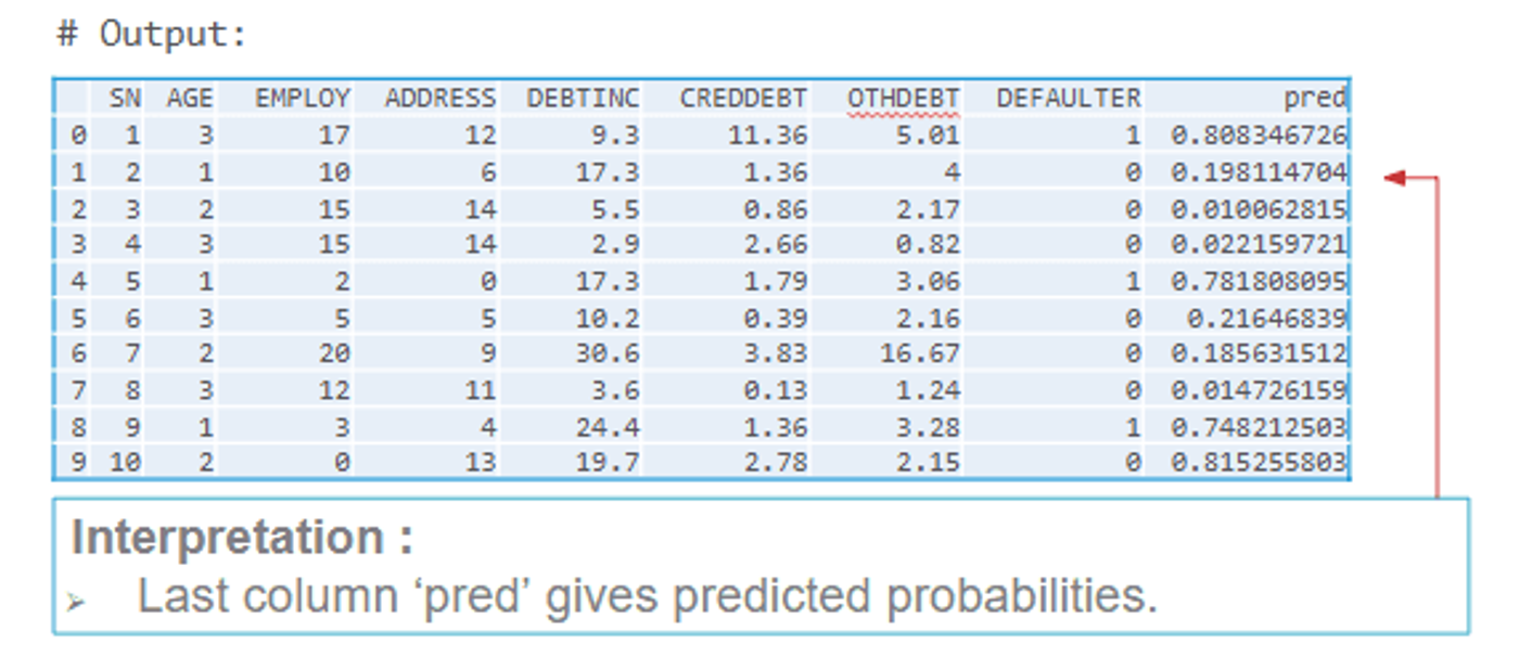

The last column in bankloan now holds these predicted probabilities.

Classification Table

To measure how well the model performs, we set a cutoff (threshold) for classifying whether a loan defaults or not. Often, we start with a threshold of 0.5:

1. If the predicted probability > 0.5, we classify the customer as a “defaulter” (1).
2. Otherwise, classify as “not defaulter” (0).

We then compare these predictions to the actual observed values (defaulters vs. not defaulters). This forms the classification table (also called a confusion matrix). The accuracy rate is the percentage of correct predictions, while the misclassification rate is the percentage of incorrect predictions.

Classification Table Terminology

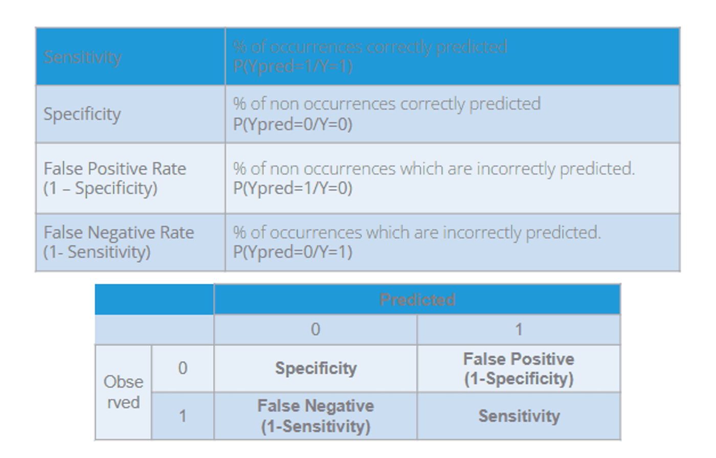
• Sensitivity: The percentage of correctly predicted events (defaulters). Mathematically, it is TP / (TP + FN).
• Specificity: The percentage of correctly predicted non-events (non-defaulters). Mathematically, it is TN / (TN + FP).
• False Positive Rate: The percentage of non-events wrongly predicted as events.
• False Negative Rate: The percentage of events wrongly predicted as non-events.

Sensitivity and Specificity Calculations

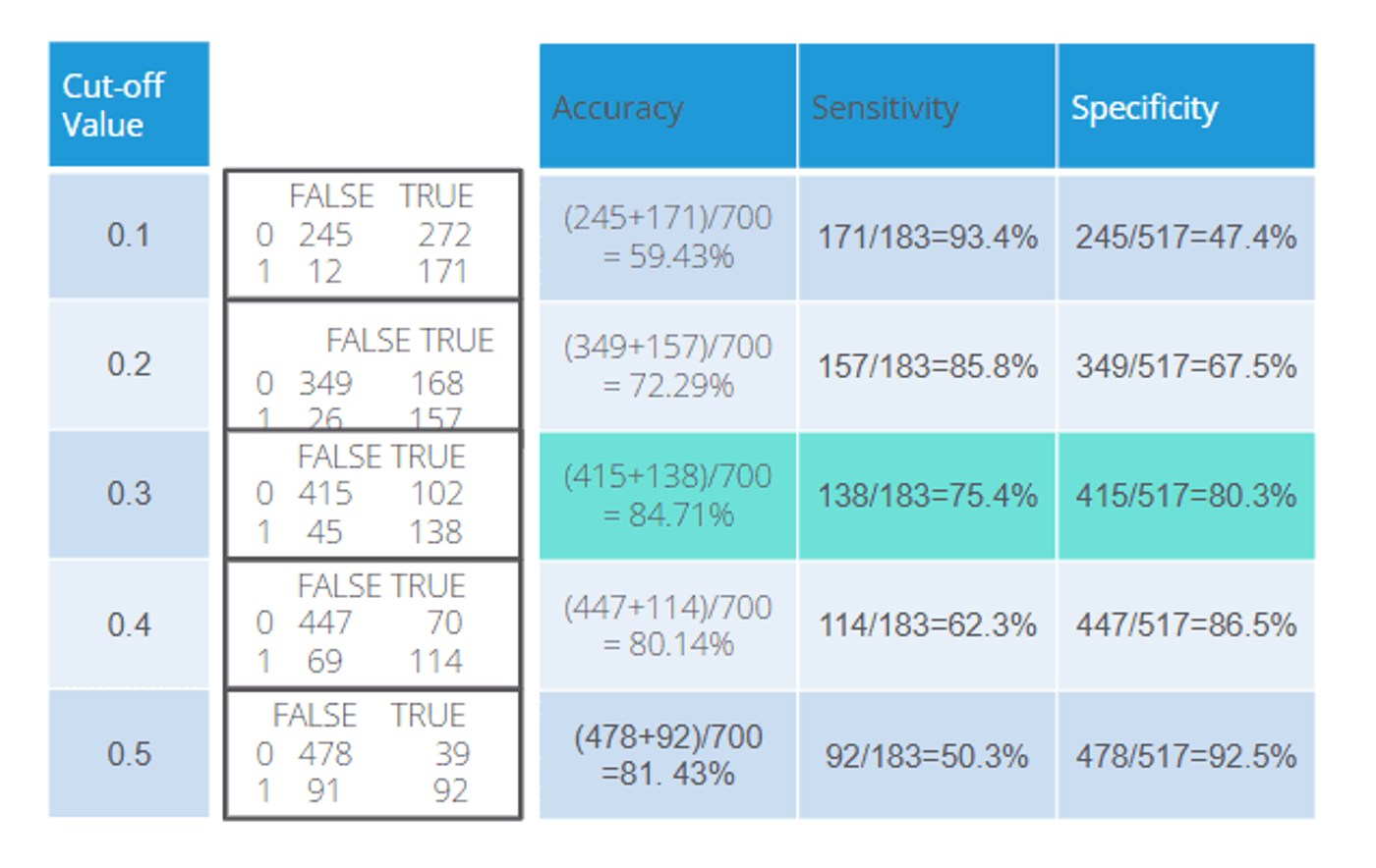
Different threshold values can yield different levels of accuracy, sensitivity, and specificity. You can compare these values for various cutoffs (e.g., 0.3, 0.4, 0.5) to choose the best threshold.

Classification Table in Python

Let’s generate the confusion matrix in Python:

from sklearn.metrics import confusion_matrix
import numpy as np

predicted_values1 = riskmodel.predict()
threshold = 0.5
predicted_class1 = np.zeros(predicted_values1.shape)
predicted_class1[predicted_values1 > threshold] = 1

cm1 = confusion_matrix(bankloan['DEFAULTER'], predicted_class1)
print('Confusion Matrix : \n', cm1)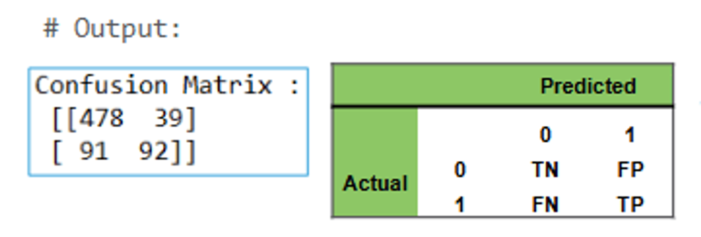

The confusion matrix (classification table) compares observed defaulters (1) vs. predicted defaulters (1), and observed non-defaulters (0) vs. predicted non-defaulters (0).

Sensitivity and Specificity in Python

sensitivity = cm1[1,1] / (cm1[1,0] + cm1[1,1])
print('Sensitivity : ', sensitivity)

specificity = cm1[0,0] / (cm1[0,0] + cm1[0,1])
print('Specificity : ', specificity)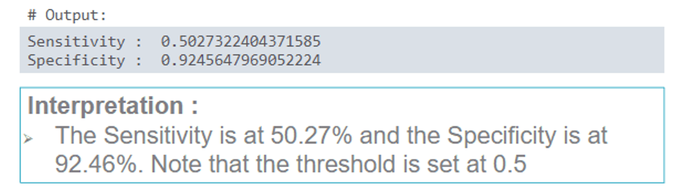

If the sensitivity is low (e.g., 50.27%), you might try adjusting the threshold to improve the model’s ability to detect defaulters (true positives).

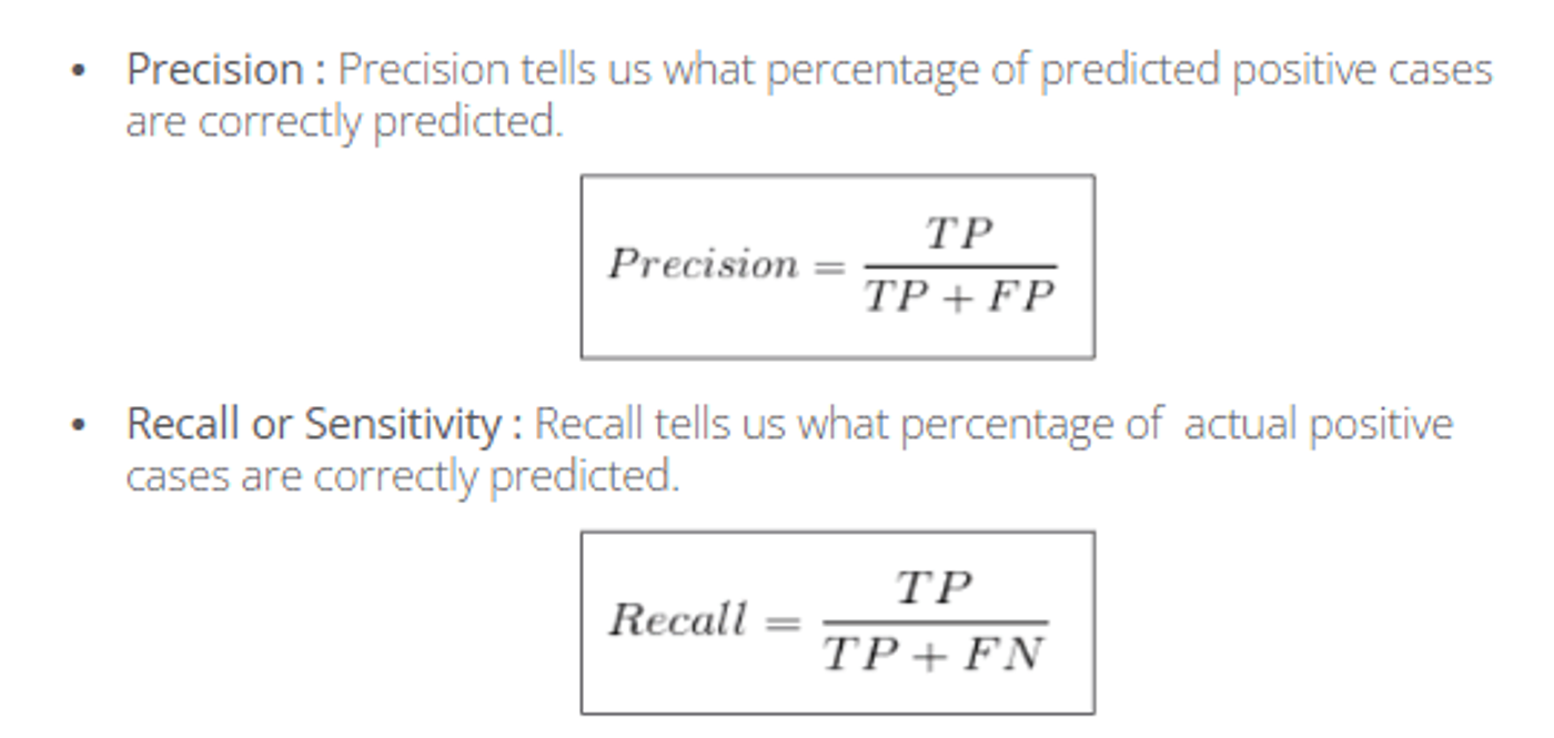
Precision & Recall

• Precision: Of the predicted positive cases, what proportion was truly positive?
• Recall: Of the actual positive cases, what proportion was predicted correctly?

These metrics are routinely used to evaluate classification models.

Classification Report

The classification_report function in Python provides recall, precision, and accuracy, all in one place:

from sklearn.metrics import classification_report

print(classification_report(bankloan['DEFAULTER'], predicted_class1))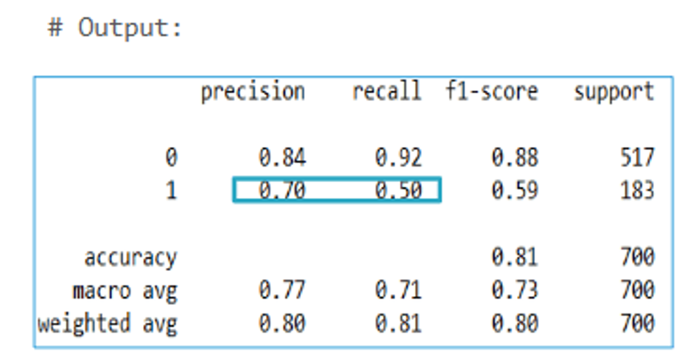

Interpretation:

• Recall is 50% & Precision is 70%.
• Accuracy is 81%.

This gives us a quick overview of how well the model is classifying defaulters and non-defaulters.

Quick Recap

We introduced how binary logistic regression models the probability of a binary outcome and applied it to a real-world banking case study aiming to predict loan defaults. Using Python, we demonstrated how to import and inspect the data, fit an initial logistic regression model, identify significant variables via p-values, and refine the model by including only those significant variables. We then showed how to calculate and interpret odds ratios, predicted probabilities, classification tables, sensitivity, specificity, precision, and recall. Altogether, this provides a comprehensive blueprint for performing binary logistic regression in Python and effectively interpreting the resulting classification model.

Key takeaways

• Binary logistic regression predicts the probability that a binary dependent variable takes the value 1; its parameters are usually estimated by maximum likelihood.
• Convert categorical variables such as age group to a category type, or Python will treat them as continuous.
• After refitting with the significant variables (EMPLOY, ADDRESS, DEBTINC and CREDDEBT), odds ratios show each variable's effect; a variable whose confidence interval excludes 1 is significant.
• At a 0.5 threshold the model's accuracy is 81%, but its recall is only 50% (precision 70%), so the threshold can be adjusted to find more defaulters.