Binary Logistic Regression in R

Binary logistic regression is a widely used statistical technique for predicting binary outcomes—situations where there are only two possibilities, such as “success” or “failure,” “yes” or “no,” or “default” versus “no default.” Unlike linear regression, which produces a continuous numeric outcome, binary logistic regression leverages a logistic function to estimate the probability of an event occurring. This makes it particularly useful for many real-world problems, including credit risk analysis, customer churn forecasting, and medical diagnoses, where the target variable only takes one of two discrete values.

In this blog, we illustrate binary logistic regression using a loan default scenario. Suppose a bank wants to develop a model to predict which customers are likely to default on their loans. The dependent variable Y (defaulter status) is 1 if the customer actually defaults and 0 otherwise. We have several independent variables: age group, years at current address, years at current employer, debt-to-income ratio, credit card debt, and other debts. By modeling and interpreting the influence of these predictors, the bank can better identify high-risk borrowers and make more informed decisions about loan approvals.

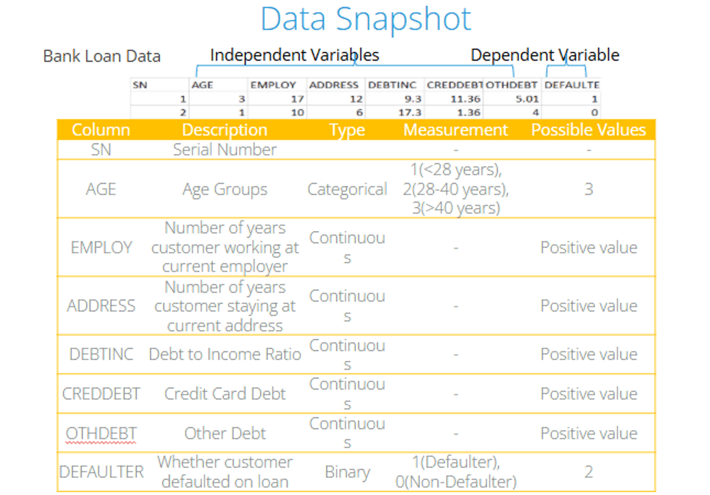
Data Snapshot

Below is a high-level look at the data. The bank’s aim is to identify significant predictors of default to guide loan disbursement decisions.

Importing the Data in R

First, we import the data and check its structure. As usual, we use the read.csv() function. Since age is a categorical variable, we need to convert it into a factor using factor().

# Import the data and check the data structure
data <- read.csv("BANK LOAN.csv", header = TRUE)
str(data)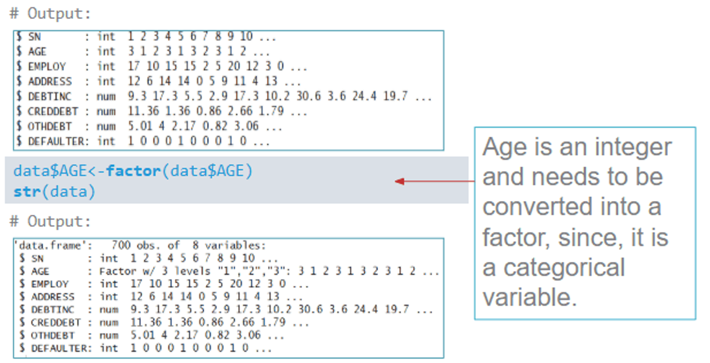

The output shows the data frame structure, helping us confirm the types of each variable.

Logistic Regression in R

Logistic regression is a form of generalized linear model (GLM). In R, we use the glm() function with the argument family=binomial to fit a binary logistic regression.

riskmodel <- glm(DEFAULTER ~ AGE + EMPLOY + ADDRESS + DEBTINC + CREDDEBT + OTHDEBT,
                 family = binomial, data = data)

• glm stands for Generalized Linear Model
• DEFAULTER is the dependent variable on the left of ~
• The independent variables (AGE, EMPLOY, ADDRESS, DEBTINC, CREDDEBT, and OTHDEBT) are separated by +
• Setting family = binomial tells R to perform a logistic regression

Individual Hypothesis Testing in R

After fitting the model, we can perform individual hypothesis testing (i.e., check which independent variables significantly impact default status). We simply use summary() on the model object.

summary(riskmodel)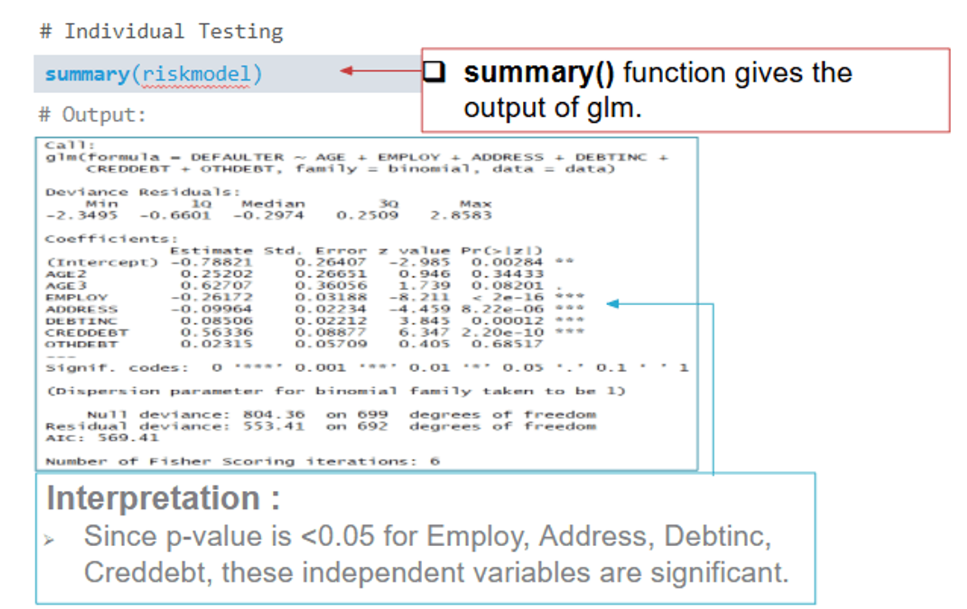

In the resulting output, we look for variables whose p-values are below 0.05. Here, EMPLOY, ADDRESS, DEBTINC, and CREDDEBT are found to be significant.

Re-run the Model in R

We then refit the model using only the significant variables.

riskmodel <- glm(DEFAULTER ~ EMPLOY + ADDRESS + DEBTINC + CREDDEBT,
                 family = binomial, data = data)

summary(riskmodel)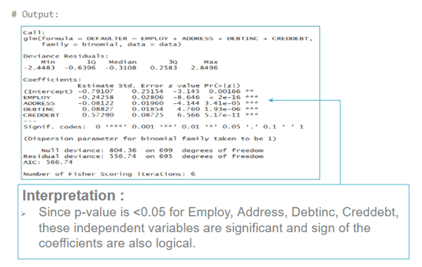

All independent variables here are statistically significant, and the signs of their coefficients align with business logic. This refined model is our candidate for further diagnostics.

Final Model

When we substitute the parameter estimates into the logistic equation, we get our final binary logistic regression model, which can be used to predict the probability of default given new values of the predictors.

Odds Ratio in R

We use the odds ratio to measure the association between each predictor and the likelihood of default. In R, we can extract the coefficients with coef(), take the exponential to get the odds ratio, and use confint() for confidence intervals.

coef(riskmodel)
exp(coef(riskmodel))
exp(confint(riskmodel))

cbind(
  coef(riskmodel),
  odds_ratio = exp(coef(riskmodel)),
  exp(confint(riskmodel))
)

• coef(riskmodel) obtains the model coefficients
• exp(coef(riskmodel)) yields the odds ratios
• exp(confint(riskmodel)) calculates confidence intervals for those odds ratios

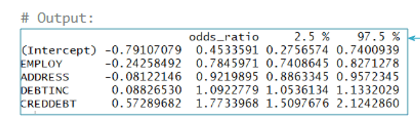
From the output, if the confidence interval for a variable’s odds ratio does not include 1, that variable is significant. For instance, if the odds ratio for CREDDEBT is around 1.77, then for a one-unit increase in credit card debt, the odds of default rise by a factor of 1.77 (all else being equal).

Predicting Probabilities in R

We can predict probabilities from the final model using the fitted() function, then round them to two decimals using round().

# Predicting Probabilities
data$predprob <- round(fitted(riskmodel), 2)
head(data, n = 10)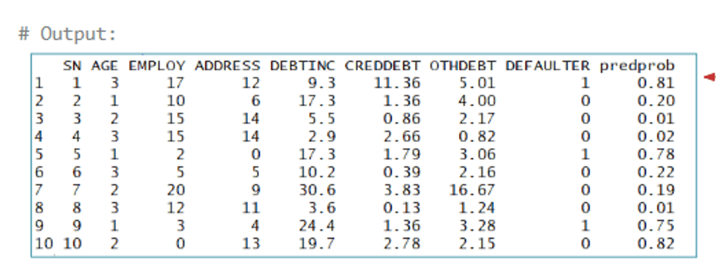

The new column predprob in the dataset contains the predicted probability of default for each observation.

Classification Table

To assess model performance, we often use a classification table based on a probability cutoff (commonly 0.5). Observations with predicted probability above the cutoff are classified as defaulters, and below it as non-defaulters.

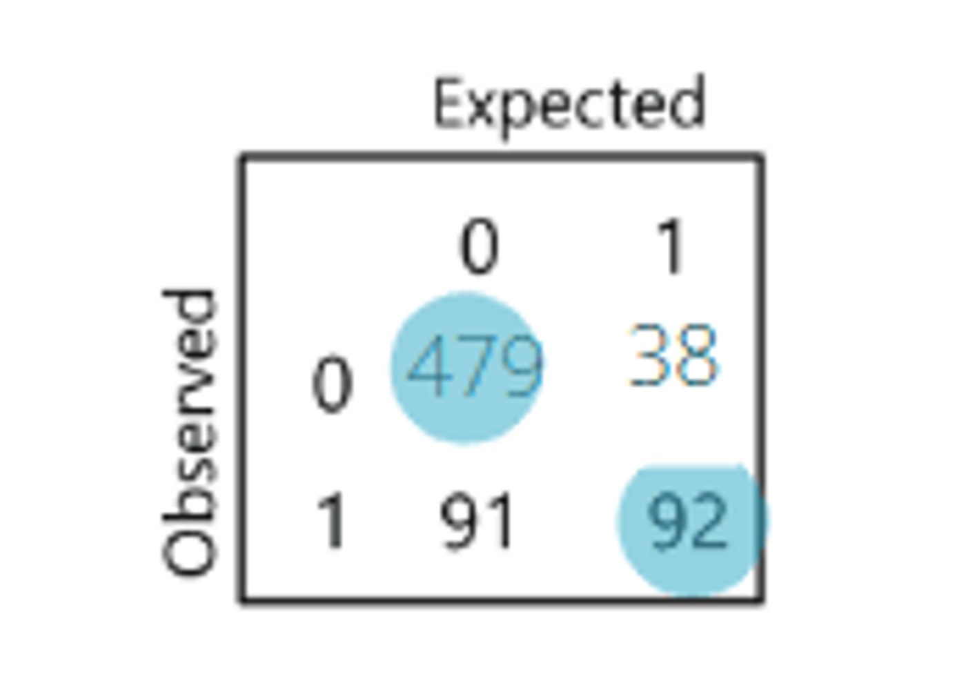
For example, if the model correctly predicts 479 of the actual non-defaulters (0) and 92 of the actual defaulters (1), the accuracy is:

(479 + 92) / 700 ≈ 81.57%

The misclassification rate is the percentage of incorrectly predicted cases. Here, it would be:

(38 + 91) / 700 ≈ 18.43%

Classification Table Terminology

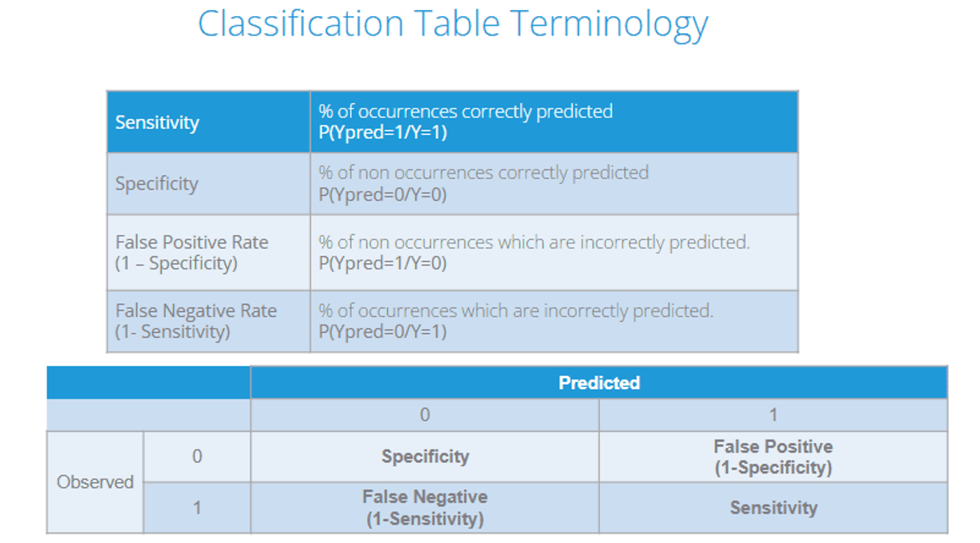
• Sensitivity: The percentage of correctly predicted defaulters (events).
• Specificity: The percentage of correctly predicted non-defaulters (non-events).
• False Positive Rate: The percentage of non-events predicted as events.
• False Negative Rate: The percentage of events predicted as non-events.

Sensitivity and Specificity

This table shows accuracy, sensitivity, and specificity for different probability cutoffs. The best cutoff is often chosen to balance both.

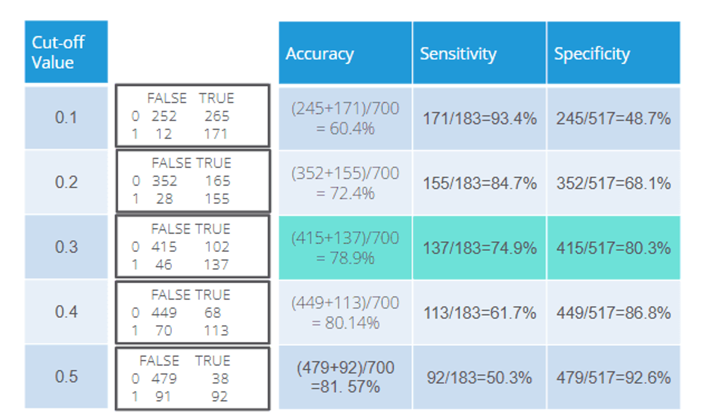
Classification and Sensitivity/Specificity Table in R

# Classification Table
classificationtable <- table(data$DEFAULTER, data$predprob > 0.5)
classificationtable

• TRUE = predicted defaulter
• FALSE = predicted non-defaulter

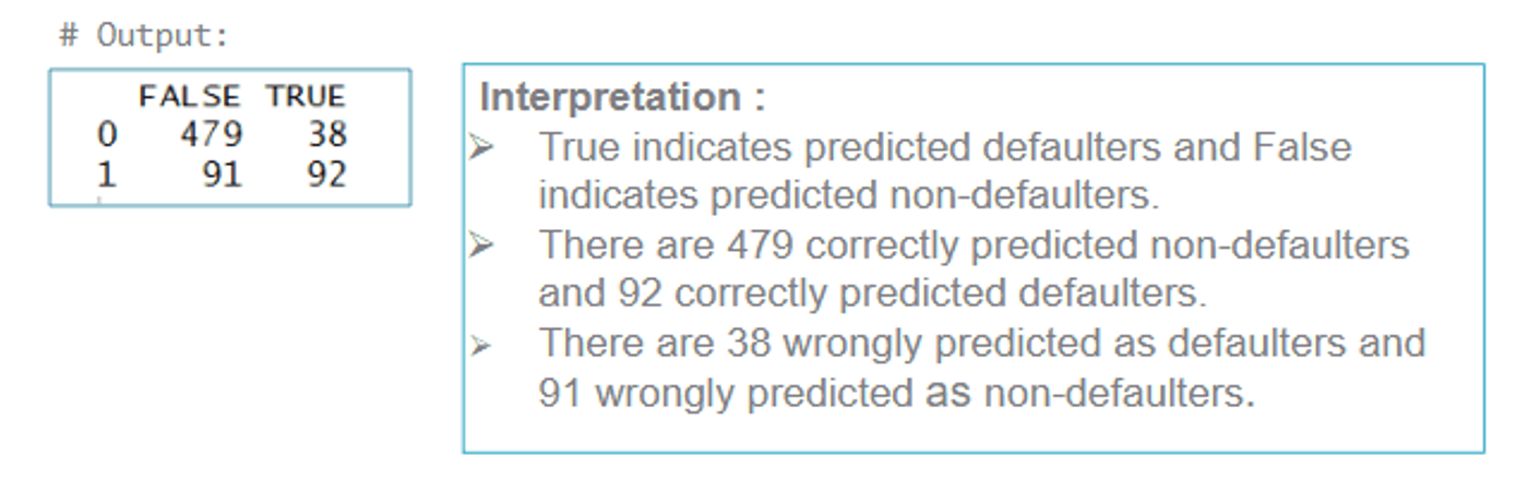
Sensitivity and Specificity in R

Finally, we compute sensitivity and specificity using the formulae:

# Sensitivity and Specificity
sensitivity <- (classificationtable[2,2] / (classificationtable[2,2] + classificationtable[2,1])) * 100
sensitivity

specificity <- (classificationtable[1,1] / (classificationtable[1,1] + classificationtable[1,2])) * 100
specificity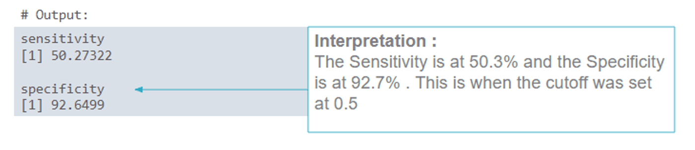

The sensitivity is around 50.3%, whereas specificity is around 92.7%, for a cutoff of 0.5. If higher sensitivity is required, we can lower the cutoff and reevaluate.

Quick Recap

In this blog, we covered how to perform binary logistic regression in R. We assessed model performance using various metrics, notably sensitivity and specificity. Sensitivity captures how well the model identifies actual defaulters, while specificity measures how accurately it identifies non-defaulters.

Key takeaways

• Binary logistic regression estimates the probability of an outcome that has only two possible values, such as default or no default.
• In R, glm() with family = binomial fits the model. In the loan case study, EMPLOY, ADDRESS, DEBTINC and CREDDEBT are significant, so the model is refitted with only those four.
• Exponentiating the coefficients gives odds ratios: an odds ratio of about 1.77 for CREDDEBT means each one-unit increase in credit card debt multiplies the odds of default by 1.77.
• At a 0.5 cut-off the model's sensitivity is about 50.3% and its specificity about 92.7%; lowering the cut-off can raise sensitivity if more defaulters need to be found.