Multiple Linear Regression in Python

Multiple Linear Regression (MLR) is the backbone of predictive modeling and machine learning. An in-depth knowledge of MLR is critical in the predictive modeling world.

Previously, we discussed implementing multiple linear regression in R. Now, we’ll look at implementing multiple linear regression using Python.

In this blog, we focus on estimating model parameters to fit a model in Python and then interpreting the results. We will use the same case study from the MLR - R to explain the Python code.

What is Multiple Linear Regression?

Multiple linear regression is used to explain the relationship between one continuous dependent variable and two or more independent variables.

For example, if the price of a house (in US dollars) is our dependent (target) variable, its size, location, air quality index, distance from the airport, and so on can be our independent variables. We call the price of the house the dependent variable.

Statistical Model for MLR

The statistical model for MLR has two parts:

• The left-hand side has the dependent variable, Y
• The right-hand side has independent variables, X1, X2, …. Xp

Each independent variable has a specific weight (coefficient) called a regression parameter b1, b2, … bp. The parameter b0 is the intercept in the model. These parameters are estimated using the Least Square Method.

Multiple Linear Regression Case Study – Modeling Job Performance Index

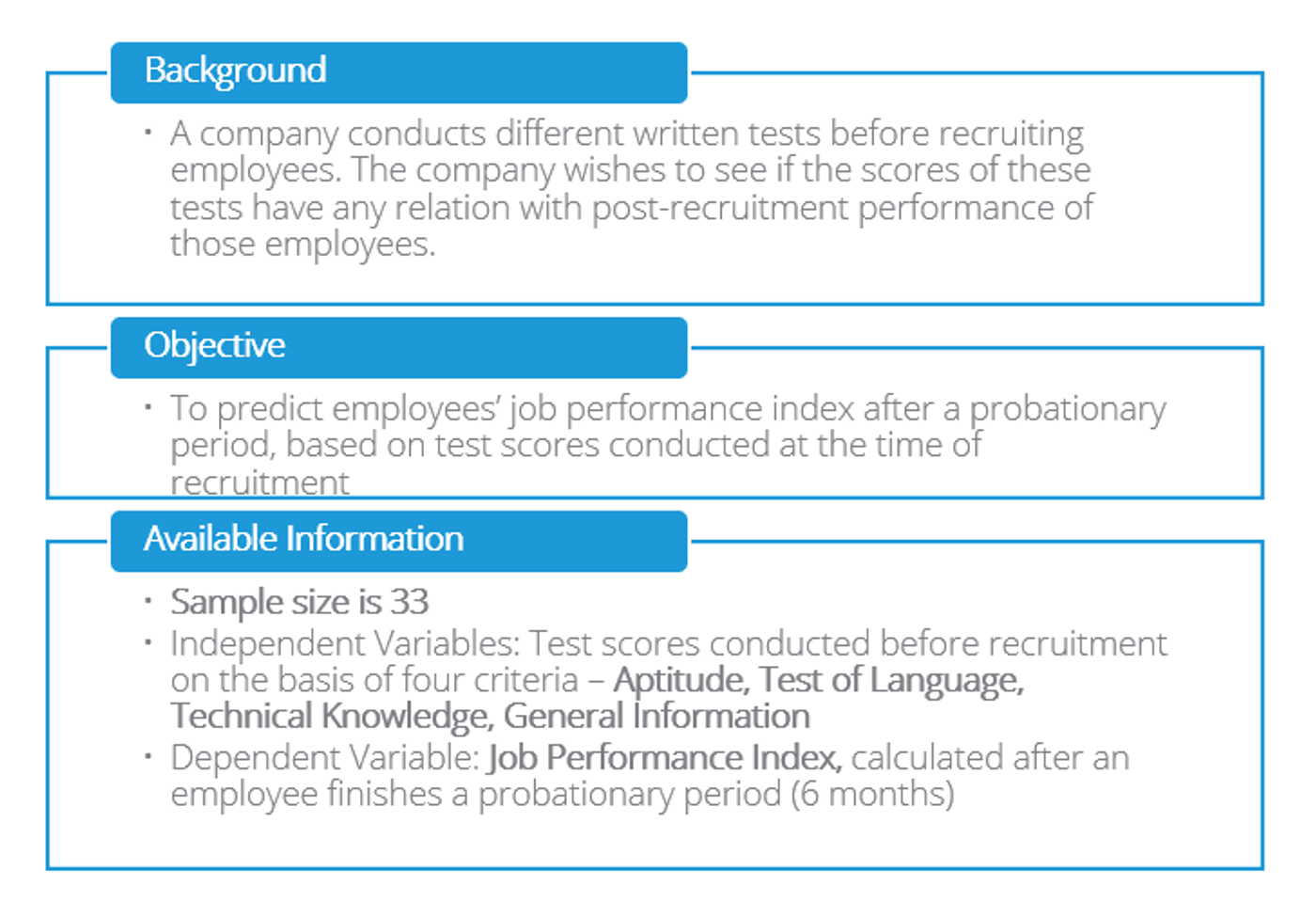
Let’s illustrate these concepts using a case study. The objective is to model the Job Performance Index (dependent variable) based on various test scores (independent variables) of newly recruited employees. The independent variables are aptitude, language test score, technical knowledge, and general information.

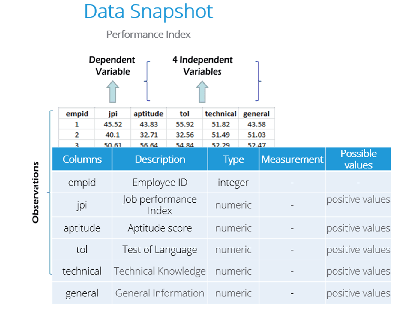
Multiple Linear Regression Dataset Snapshot

Here is a snapshot of the data showing our dependent and independent variables. All variables are numeric. The “Employee ID” column is not used in the model.

Graphical Representation of Data

It is advisable to have a graphical view of the data through scatter plots to understand bivariate relationships between variables. We import the example data with the read_csv function (from pandas) and then use the seaborn library’s pairplot to visualize these relationships.

# importing the Data
import pandas as pd
import seaborn as sns

perindex = pd.read_csv("Performance Index.csv")

# Graphical Representation of the Data
sns.pairplot(perindex)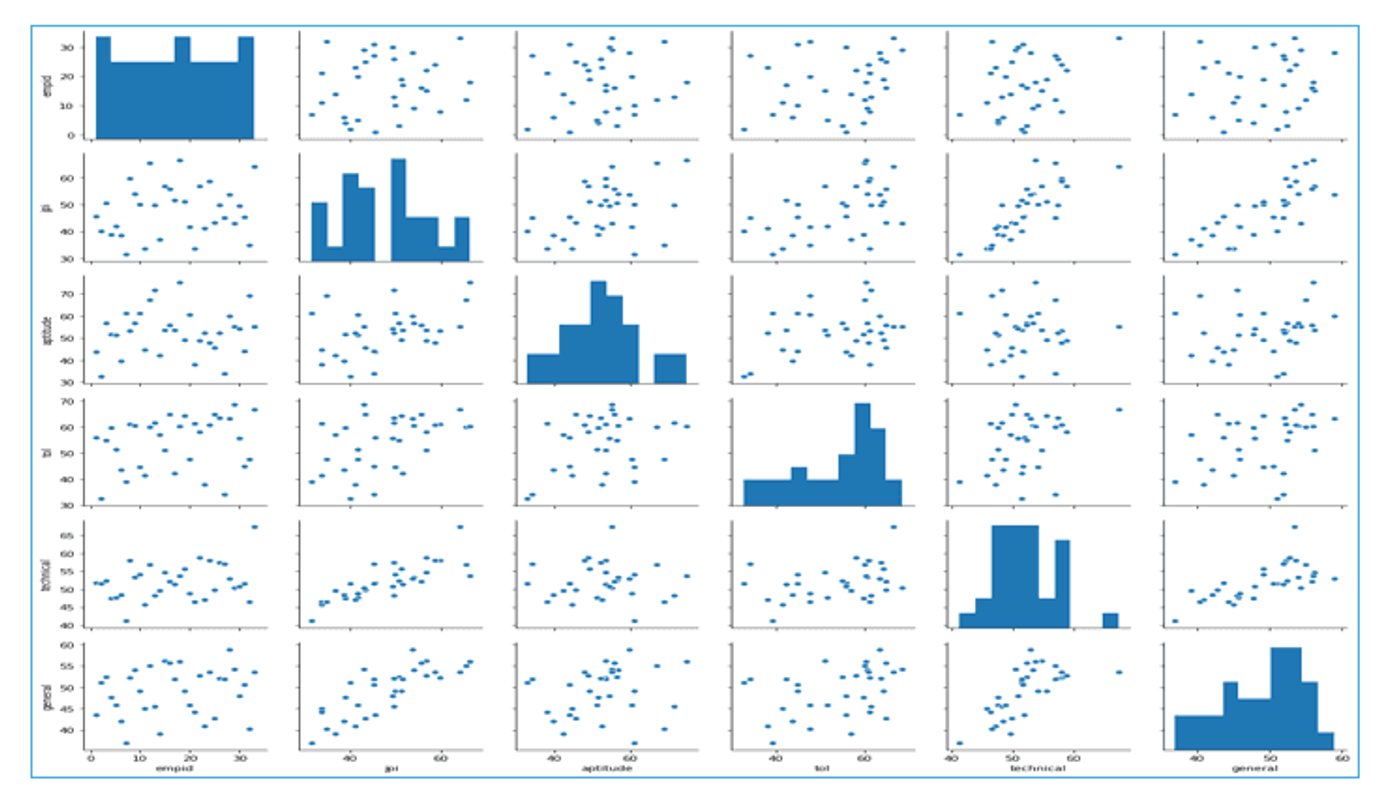

The scatter plot matrix helps visualize bivariate relationships among variables and also shows the distribution of each variable (histograms on the diagonal). We can observe that the Job Performance Index has a high correlation with Technical Knowledge and General Information scores.

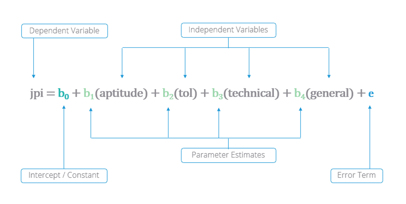
Model for the Case Study

where

• b0 is the intercept (constant).
• b1, b2, b3, b4 are our parameter estimates for each independent variable.
• ε is the error term.

Parameter Estimation Using the Least Square Method

Parameters (b0, b1, b2, b3, b4) are estimated using the Least Square Method. Once they are estimated, we have a fully specified model equation.

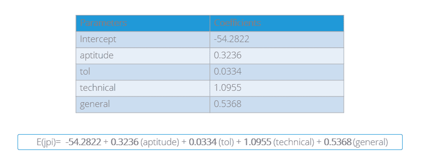
Parameter Estimation Using ols() Function in Python

We use the statsmodels library (aliased as smf). The ols function (Ordinary Least Squares) fits our regression model, requiring a formula that specifies dependent and independent variables. The data for the model is passed through the data argument.

# Model Fit
import statsmodels.formula.api as smf

jpimodel = smf.ols('jpi ~ tol + aptitude + technical + general', data=perindex).fit()
print(jpimodel.params)

• ols() fits a linear regression model.
• The tilde (~) separates the dependent variable on the left from the independent variables on the right.
• Independent variables are separated by the plus (+) sign.

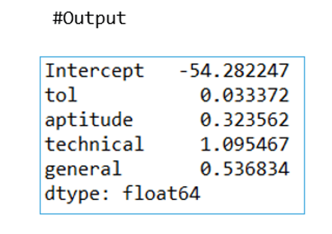
Interpretation:

• jpimodel.params prints the parameter estimates.
• The sign (positive/negative) of each parameter indicates the direction of the relationship with the dependent variable.

Interpretation of Partial Regression Coefficients

For each one-unit increase in an independent variable X, the expected value of Y changes by the corresponding parameter estimate b, holding all other variables constant.

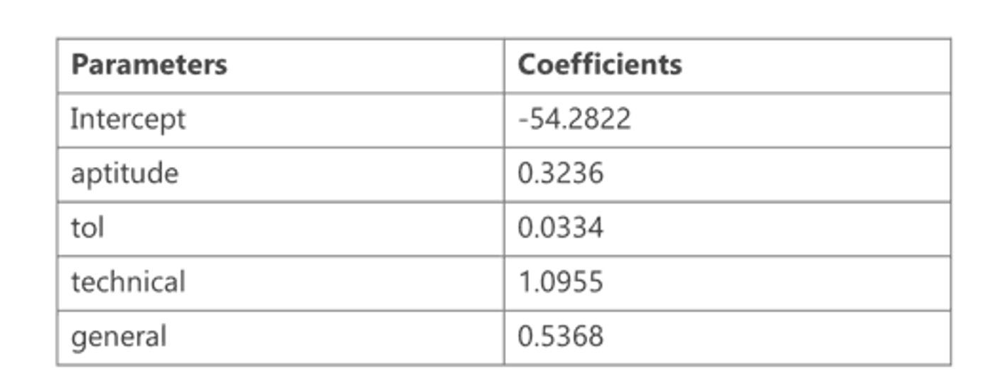
For example, if the parameter estimate for Aptitude is 0.32, then a one-unit increase in Aptitude score is associated with a 0.32 point increase in the Job Performance Index, on average, assuming all other factors remain unchanged.

Key takeaways

• A scatter plot matrix shows bivariate relationships at a glance: here, the Job Performance Index correlates highly with Technical Knowledge and General Information scores.
• smf.ols() fits an MLR model from a formula, with the dependent variable to the left of the tilde (~) and the independent variables joined by plus signs.
• The sign of each parameter estimate shows the direction of its relationship with the dependent variable.
• A partial regression coefficient is the expected change in Y for a one-unit increase in X, holding all other variables constant: an Aptitude estimate of 0.32 means 0.32 more points on the Job Performance Index per point of Aptitude.

Having walked through the Python implementation, you should now have a clearer idea of how to set up, estimate, and interpret a multiple linear regression model in Python.